This is a demonstration that uses R and statistics to solve the marketing problem outlined below.
I am using Windows 10, R version 4.1.0, and RStudio version 1.4.1106.
The data for this project can be found here Marketing Analytics: Practice Exploratory and Statistical Analysis with Marketing Data.
Table of Contents
- Task Details
- Section 01: Understanding the Data
- Section 02: Exploratory Data Analysis
- Section 03: Data Visualization
- Section 04: Statistical Analysis
- Main Takeaways
I will use the following packages:
# Data wrangling, data manipulation, & data visualization
library(tidyverse)

# Statistical package for ANOVAs and Linear Mixed Models
library(afex)

# Extra stats functions
library(car)

# Assumption checks for linear regression
library(gvlma)

# Machine learning package
library(caret)

# Formatting package
library(knitr)

# Knitr Kable Extras
library(kableExtra)

# Plotting extras
library(gridExtra)
Task Details
You’re a marketing analyst and you’ve been told by the Chief Marketing Officer that recent marketing campaigns have not been as effective as they were expected to be. You need to analyze the data set to understand this problem and propose data-driven solutions.
There are five sections to this task:
- Understanding the Data
- Exploratory Data Analysis
- Data Visualization
- Statistical Analysis
Section 01: Understanding the Data
Reading and viewing the data
# Load the data
mkt_data_orig <- read_csv("marketing_data.csv")

# View the data we are using
str(mkt_data_orig, give.attr = FALSE)
## spec_tbl_df [2,240 x 28] (S3: spec_tbl_df/tbl_df/tbl/data.frame)
##  $ ID                 : num [1:2240] 1826 1 10476 1386 5371 ...
##  $ Year_Birth         : num [1:2240] 1970 1961 1958 1967 1989 ...
##  $ Education          : chr [1:2240] "Graduation" "Graduation" "Graduation" "Graduation" ...
##  $ Marital_Status     : chr [1:2240] "Divorced" "Single" "Married" "Together" ...
##  $ Income             : chr [1:2240] "$84,835.00" "$57,091.00" "$67,267.00" "$32,474.00" ...
##  $ Kidhome            : num [1:2240] 0 0 0 1 1 0 0 0 0 0 ...
##  $ Teenhome           : num [1:2240] 0 0 1 1 0 0 0 1 1 1 ...
##  $ Dt_Customer        : chr [1:2240] "6/16/14" "6/15/14" "5/13/14" "5/11/14" ...
##  $ Recency            : num [1:2240] 0 0 0 0 0 0 0 0 0 0 ...
##  $ MntWines           : num [1:2240] 189 464 134 10 6 336 769 78 384 384 ...
##  $ MntFruits          : num [1:2240] 104 5 11 0 16 130 80 0 0 0 ...
##  $ MntMeatProducts    : num [1:2240] 379 64 59 1 24 411 252 11 102 102 ...
##  $ MntFishProducts    : num [1:2240] 111 7 15 0 11 240 15 0 21 21 ...
##  $ MntSweetProducts   : num [1:2240] 189 0 2 0 0 32 34 0 32 32 ...
##  $ MntGoldProds       : num [1:2240] 218 37 30 0 34 43 65 7 5 5 ...
##  $ NumDealsPurchases  : num [1:2240] 1 1 1 1 2 1 1 1 3 3 ...
##  $ NumWebPurchases    : num [1:2240] 4 7 3 1 3 4 10 2 6 6 ...
##  $ NumCatalogPurchases: num [1:2240] 4 3 2 0 1 7 10 1 2 2 ...
##  $ NumStorePurchases  : num [1:2240] 6 7 5 2 2 5 7 3 9 9 ...
##  $ NumWebVisitsMonth  : num [1:2240] 1 5 2 7 7 2 6 5 4 4 ...
##  $ AcceptedCmp3       : num [1:2240] 0 0 0 0 1 0 1 0 0 0 ...
##  $ AcceptedCmp4       : num [1:2240] 0 0 0 0 0 0 0 0 0 0 ...
##  $ AcceptedCmp5       : num [1:2240] 0 0 0 0 0 0 0 0 0 0 ...
##  $ AcceptedCmp1       : num [1:2240] 0 0 0 0 0 0 0 0 0 0 ...
##  $ AcceptedCmp2       : num [1:2240] 0 1 0 0 0 0 0 0 0 0 ...
##  $ Response           : num [1:2240] 1 1 0 0 1 1 1 0 0 0 ...
##  $ Complain           : num [1:2240] 0 0 0 0 0 0 0 0 0 0 ...
##  $ Country            : chr [1:2240] "SP" "CA" "US" "AUS" ...
# Get the dimensions
mkt_dim <- dim(mkt_data_orig)
The data is from 2240 customers with 28 variables per customer.
Data transformation
- The Income variable is a character data type and needs to be numeric.
- The Year_Birth variable can be converted to an age variable for better interpretation.
- The Dt_Customer (Date) variable is a character data type that can be turned into a date.
# Transform the data - Create a new data frame
mkt_data <- mkt_data_orig %>%
  mutate(Income = str_remove_all(Income, pattern = "[$,]"),
         Income = as.numeric(Income), # Change Income to numeric
         Age    = lubridate::year(Sys.Date()) - Year_Birth, # Create the Age variable from Year_Birth
         Dt_Customer = as.Date(Dt_Customer, "%m/%d/%y")) # Convert to a Date format
Similar to transforming the age variable, we can also calculate a variable that represents the number of years a person was a customer.
We can also create a categorical variable that categorizes people by generation.
For example:
- The Silent Generation: 1925 - 1945
- Baby Boomers: 1946 - 1964
- Gen X: 1965 - 1979
- Millennials: 1980 - 1996
# Create the number of years a person was a customer
mkt_data <- mkt_data %>%
  mutate(Yr_Customer = lubridate::year(Sys.Date()) - lubridate::year(Dt_Customer)) # Extract the year from Dt_Cusomter and subtract it from 2021

# Create a variable for the generation
# First get the min and max year date to see where we should start and end
min(mkt_data$Year_Birth) # 1940
## [1] 1893
max(mkt_data$Year_Birth) # 1996
## [1] 1996
mkt_data <- mkt_data %>%
  mutate(Generation = case_when(
    Year_Birth >= 1925 & Year_Birth <= 1945 ~ "Silent",
    Year_Birth >= 1946 & Year_Birth <= 1964 ~ "Boomer",
    Year_Birth >= 1965 & Year_Birth <= 1979 ~ "Gen-X",
    Year_Birth >= 1980 & Year_Birth <= 1996 ~ "Millenial"
  ))
Section 02: Exploratory Data Analysis
Are there any outliers? How will you wrangle/handle them?
To find out what the outliers are, I need to reduce the data set to just the numeric data. The numeric data are:
- Income
- Age
- Kidhome
- Teenhome
- Recency
- Mnt* - Amount spent
- Num*Purchases - Number of Purchases
- NumWebVisitsMonth
- Accepted* - Number of accepted marketing campaigns
mkt_plot <- mkt_data %>%
  select_if(is.numeric) %>% # Only select the numeric data
  select(-ID, -Response) # Remove ID

mkt_plot %>%
  pivot_longer(everything(), names_to = "variable", values_to = "response") %>% # Wide -> Long
  ggplot(aes(x = variable, y = response)) + # Set up the aesthetic and plot
  geom_boxplot(width = 0.1) + # Create box plots
  facet_wrap(. ~ variable, scale = "free", ncol = 6) + # Show box plots in a grid
  theme_classic() +
  theme(strip.text.x = element_blank())
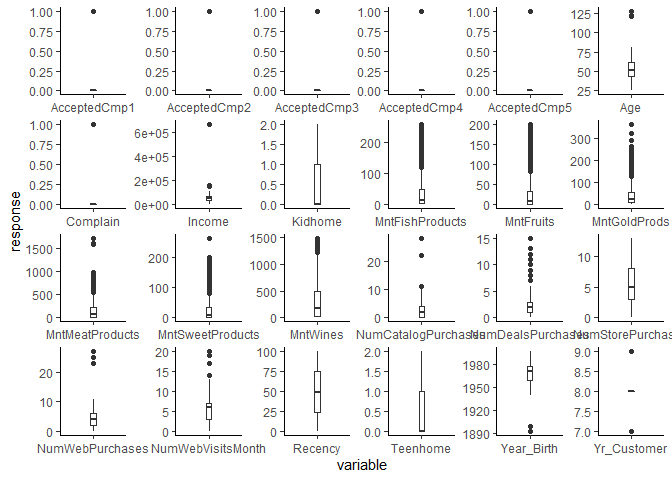
There are some outliers in the Age variable (top right boxplot) - there seems to be a few customers that are over the age of 100. That is a bit suspicious.
There are some outliers in the Income variable (2nd row, 2nd column) - there are some customers that have over $600,000 income. However, this could be true.
# Get the outliers for Age
Age_out <- boxplot.stats(mkt_data$Age)
There are 3 customers who are the ages of 128, 122, 121. We will remove these customers who are over the age of 100.
Are there any missing data? How will you wrangle/handle them?
missing_data <- mkt_data %>%
  map(~sum(is.na(.))) %>% # Get the number of NAs for each column
  unlist(.) %>% # Strip the list formatting
  as.data.frame(.) %>% # Convert to a data frame
  arrange(desc(.)) %>% # Arrange in descending order
  rename(`N Missing` = ".")

knitr::kable(missing_data)
| N Missing | |
|---|---|
| Income | 24 |
| Generation | 3 |
| ID | 0 |
| Year\_Birth | 0 |
| Education | 0 |
| Marital\_Status | 0 |
| Kidhome | 0 |
| Teenhome | 0 |
| Dt\_Customer | 0 |
| Recency | 0 |
| MntWines | 0 |
| MntFruits | 0 |
| MntMeatProducts | 0 |
| MntFishProducts | 0 |
| MntSweetProducts | 0 |
| MntGoldProds | 0 |
| NumDealsPurchases | 0 |
| NumWebPurchases | 0 |
| NumCatalogPurchases | 0 |
| NumStorePurchases | 0 |
| NumWebVisitsMonth | 0 |
| AcceptedCmp3 | 0 |
| AcceptedCmp4 | 0 |
| AcceptedCmp5 | 0 |
| AcceptedCmp1 | 0 |
| AcceptedCmp2 | 0 |
| Response | 0 |
| Complain | 0 |
| Country | 0 |
| Age | 0 |
| Yr\_Customer | 0 |
There is only missing income data for 24 people. This is only 1.0714286% of the data. We can do the following: 1. Remove the 24 customers who are missing Income data 2. Use the median Income to impute the data for the customers missing data
I will remove the following from the data: - The 24 customers who are missing Income data because it is a very small fraction of the data - The 3 customers who are over the age of 100
Let’s check out the categorical variables
mkt_data %>%
  select_if(is.character) # list out all the categorical variables
## # A tibble: 2,240 x 4
##    Education  Marital_Status Country Generation
##    <chr>      <chr>          <chr>   <chr>
##  1 Graduation Divorced       SP      Gen-X
##  2 Graduation Single         CA      Boomer
##  3 Graduation Married        US      Boomer
##  4 Graduation Together       AUS     Gen-X
##  5 Graduation Single         SP      Millenial
##  6 PhD        Single         SP      Boomer
##  7 2n Cycle   Married        GER     Boomer
##  8 Graduation Together       SP      Gen-X
##  9 PhD        Married        US      Boomer
## 10 PhD        Married        IND     Boomer
## # ... with 2,230 more rows
Let’s see the responses and # of responses in each categorical variable
- Education - Martial Status - Country - gen
Education
| Education | Frequency |
|---|---|
| 2n Cycle | 203 |
| Basic | 54 |
| Graduation | 1127 |
| Master | 370 |
| PhD | 486 |
The education variable has 5 different responses and no apparent outliers.
Marital Status
| Marital Status | Frequency |
|---|---|
| Absurd | 2 |
| Alone | 3 |
| Divorced | 232 |
| Married | 864 |
| Single | 480 |
| Together | 580 |
| Widow | 77 |
| YOLO | 2 |
The marital status variable has 8 different variables, but there are a few outliers. They will be removed from the data.
- Absurd: 2 responses
- Alone: 3 responses
- YOLO: 2 responses
Country
| Country | Frequency |
|---|---|
| AUS | 160 |
| CA | 268 |
| GER | 120 |
| IND | 148 |
| ME | 3 |
| SA | 337 |
| SP | 1095 |
| US | 109 |
The Country variable looks good, but the ME country has only 3 responses. ME will be removed from the data.
Gen
| Generation | Frequency |
|---|---|
| Boomer | 759 |
| Gen-X | 1030 |
| Millenial | 424 |
| Silent | 24 |
The gen variable also looks OK. Although the silent generation is rather low, no data will be removed.
Removing the variables
mkt_data_ana <- mkt_data %>%
  filter(!is.na(Income), Age < 100) %>% # Remove the NAs from Income and Age
  filter(!(Marital_Status %in% c("Absurd", "Alone", "YOLO"))) %>% # Remove the low variables from Marital Status
  filter(!(Country) %in% c("ME")) # Remove ME from the data
We dropped 37 customers from the analysis.
Factorizing the categorical variables
The categorical variable will transformed into factors to make sure that statistics are handled correctly.
mkt_data_ana <- mkt_data_ana %>%
  mutate(Education      = factor(Education),
         Marital_Status = factor(Marital_Status),
         Country        = factor(Country),
         Generation     = factor(Generation))
Are there any useful variables that you can engineer with the given data?
We can sum the data that is split by the different types of products, marketing campaigns accepted, purchases, and number of children.
We can also calculate the average amount spent and the average total purchases for each customer.
mkt_data_ana <- mkt_data_ana %>%
  mutate(tot_mnt      = MntWines + MntFruits + MntMeatProducts + MntFishProducts + MntSweetProducts + MntGoldProds, # total amount
         num_accepted = AcceptedCmp1 + AcceptedCmp2 + AcceptedCmp3 + AcceptedCmp4 + AcceptedCmp5, # number of marketing campaigns accepted
         tot_pur      = NumDealsPurchases + NumWebPurchases + NumCatalogPurchases + NumStorePurchases, # total number of purchases
         avg_mnt      = rowMeans(select(., starts_with("Mnt")), na.rm = TRUE),
         avg_pur      = rowMeans(select(., ends_with("Purchases")), na.rm = TRUE),
         Dependents   = factor(Teenhome + Kidhome)) # total number of dependents
Section 03: Data Visualization
Demographics visualization
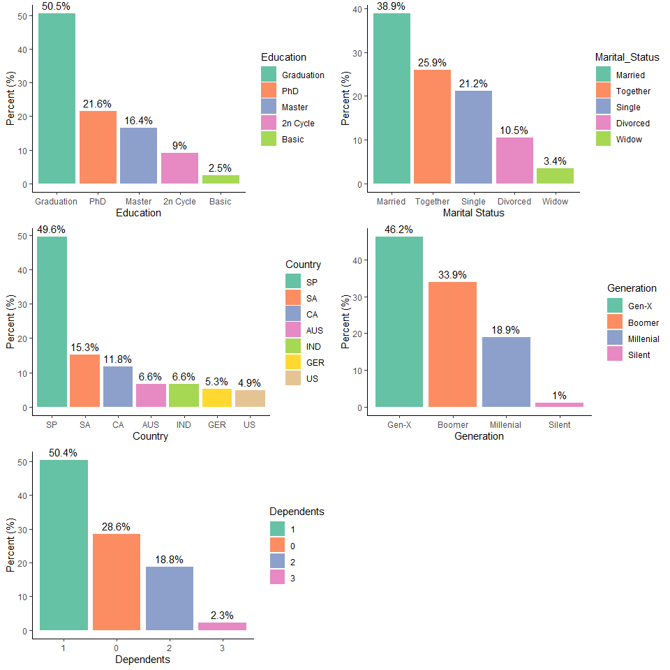
To help understand the customers, I want to see their education level, marital status, country, and generation
What does the average customer look like for this company?
Findings
- Age: 52 years old
- Has been a customer for about 8 years
- Has an income of $5.1373^{4}
- Has at least 1 dependent
- Made a purchase from the company in the last 49
- They are most likely married
- They are most likely graduated
- They are most likely from Spain
# Education Level
edu_lvl <- mkt_data_ana %>%
  count(Education) %>%
  mutate(prop = prop.table(n),
         Percent  = prop*100,
         Education = fct_reorder(Education, desc(Percent)))

# Education Plot
ed_plt <- ggplot(data = edu_lvl, aes(x = Education, y = Percent, fill = Education)) +
  geom_bar(stat = "Identity") + # Use the data from the table
  labs(x = "Education", y = "Percent (%)") + # Change the axis labels
  geom_text(aes(label = round(Percent, 1) %>% str_c("%")), vjust = -0.5) + # Add the labels to the figure
  scale_fill_brewer(palette = "Set2") + # Change the colors
  coord_cartesian(clip = "off") +
  theme_classic()

# Marital Status
m_stat <- mkt_data_ana %>%
  count(Marital_Status) %>%
  mutate(prop = prop.table(n),
         Percent  = prop*100,
         Marital_Status = fct_reorder(Marital_Status, desc(Percent)))

# Marital Status Plot
ms_plt <- ggplot(data = m_stat, aes(x = Marital_Status, y = Percent, fill = Marital_Status)) +
  geom_bar(stat = "Identity") + # Use the data from the table
  labs(x = "Marital Status", y = "Percent (%)") + # Change the axis labels
  geom_text(aes(label = round(Percent, 1) %>% str_c("%")), vjust = -0.5) + # Add the labels to the figure
  scale_fill_brewer(palette = "Set2") + # Change the colors
  coord_cartesian(clip = "off") +
  theme_classic()

# Country
cnty <- mkt_data_ana %>%
  count(Country) %>%
  mutate(prop = prop.table(n),
         Percent  = prop*100,
         Country = fct_reorder(Country, desc(Percent)))

# Country plot
cnty_plt <- ggplot(data = cnty, aes(x = Country, y = Percent, fill = Country)) +
  geom_bar(stat = "Identity") + # Use the data from the table
  labs(x = "Country", y = "Percent (%)") + # Change the axis labels
  geom_text(aes(label = round(Percent, 1) %>% str_c("%")), vjust = -0.5) + # Add the labels to the figure
  scale_fill_brewer(palette = "Set2") + # Change the colors
  coord_cartesian(clip = "off") +
  theme_classic()

# Generation
gen <- mkt_data_ana %>%
  count(Generation) %>%
  mutate(prop = prop.table(n),
         Percent  = prop*100,
         Generation = fct_reorder(Generation, desc(Percent)))

# Generation plot
gen_plt <- ggplot(data = gen, aes(x = Generation, y = Percent, fill = Generation)) +
  geom_bar(stat = "Identity") + # Use the data from the table
  labs(x = "Generation", y = "Percent (%)") + # Change the axis labels
  geom_text(aes(label = round(Percent, 1) %>% str_c("%")), vjust = -0.5) + # Add the labels to the figure
  scale_fill_brewer(palette = "Set2") + # Change the colors
  coord_cartesian(clip = "off") +
  theme_classic()

# dependents
depe <- mkt_data_ana %>%
  count(Dependents) %>%
  mutate(prop = prop.table(n),
         Percent  = prop*100,
         Dependents = fct_reorder(Dependents, desc(Percent)))

# Generation plot
depe_plt <- ggplot(data = depe, aes(x = Dependents, y = Percent, fill = Dependents)) +
  geom_bar(stat = "Identity") + # Use the data from the table
  labs(x = "Dependents", y = "Percent (%)") + # Change the axis labels
  geom_text(aes(label = round(Percent, 1) %>% str_c("%")), vjust = -0.5) + # Add the labels to the figure
  scale_fill_brewer(palette = "Set2") + # Change the colors
  coord_cartesian(clip = "off") +
  theme_classic()

# Plot the barplots in a grid
grid.arrange(ed_plt, ms_plt, cnty_plt, gen_plt, depe_plt, ncol = 2)
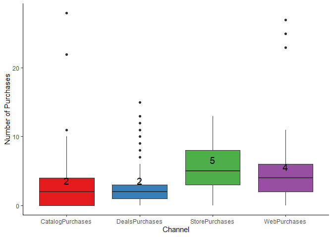
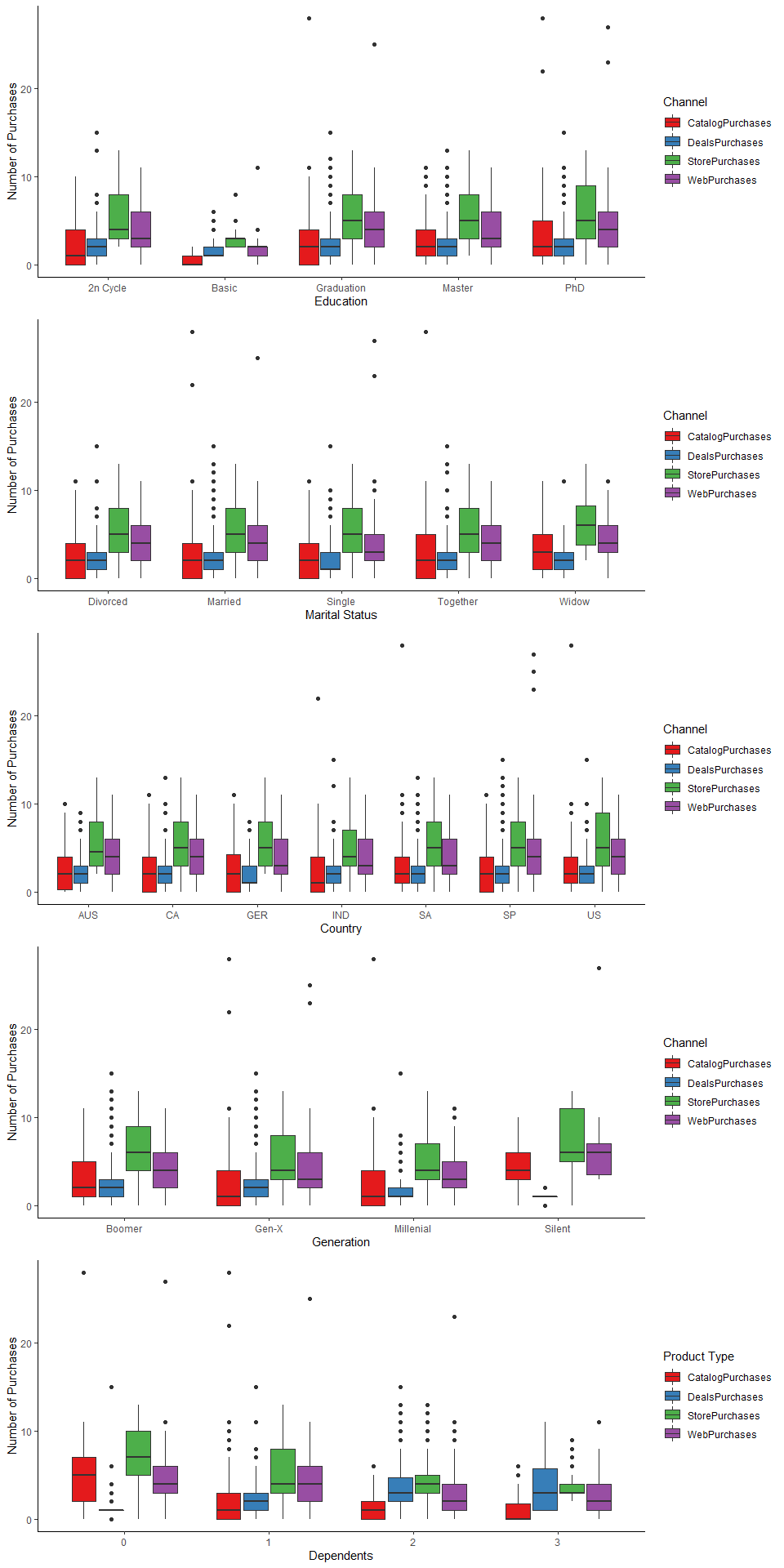
Which channels are under performing?
# Plot of channels
chan <- mkt_data_ana %>%
  select(NumWebPurchases, NumCatalogPurchases, NumStorePurchases, NumDealsPurchases) %>% # Select the education and amount spent
  pivot_longer(starts_with("Num"), names_to = "variable", values_to = "response") %>% # Wide to long format
  mutate(variable = str_remove_all(variable, "Num"))# Remove the num

chan_med <- chan %>%
  group_by(variable) %>%
  summarise(med = median(response))

c_plt <- ggplot(data = chan, aes(x = variable, y = response, fill = variable)) +
  geom_boxplot() +
  labs(x = "Channel", y = "Number of Purchases") +
  scale_fill_brewer(palette = "Set1") + # Change the colors
  geom_text(data = chan_med, aes(x = variable, y = med, label = med), size = 5,  vjust = -1) +
  coord_cartesian(clip = "off") +
  theme_classic() +
  theme(legend.position = "none")

c_plt
# Spending by education
ed_chan <- mkt_data_ana %>%
  select(Education, NumWebPurchases, NumCatalogPurchases, NumStorePurchases, NumDealsPurchases) %>% # Select the education and amount spent
  group_by(Education) %>% # Group by Education
  pivot_longer(starts_with("Num"), names_to = "variable", values_to = "response") %>% # Wide to long format
  mutate(variable = str_remove_all(variable, "Num"))# Remove the num

ed_c_plt <- ggplot(data = ed_chan, aes(x = Education, y = response, fill = variable)) +
  geom_boxplot() +
  labs(x = "Education", y = "Number of Purchases", fill = "Channel") +
  scale_fill_brewer(palette = "Set1") + # Change the colors +
  coord_cartesian(clip = "off") +
  theme_classic()

# Spending by Marital Status
ms_chan <- mkt_data_ana %>%
  select(Marital_Status, NumWebPurchases, NumCatalogPurchases, NumStorePurchases, NumDealsPurchases) %>% # Select the ms and amount spent
  group_by(Marital_Status) %>% # Group by Education
  pivot_longer(starts_with("Num"), names_to = "variable", values_to = "response") %>% # Wide to long format
  mutate(variable = str_remove_all(variable, "Num"))# Remove the num

ms_c_plt <- ggplot(data = ms_chan, aes(x = Marital_Status, y = response, fill = variable)) +
  geom_boxplot() +
  labs(x = "Marital Status", y = "Number of Purchases", fill = "Channel") +
  scale_fill_brewer(palette = "Set1") +
  coord_cartesian(clip = "off") +
  theme_classic()

# Spending by Country
ctr_chan <- mkt_data_ana %>%
  select(Country, NumWebPurchases, NumCatalogPurchases, NumStorePurchases, NumDealsPurchases) %>% # Select the country and amount spent
  group_by(Country) %>% # Group by Marital_Status
  pivot_longer(starts_with("Num"), names_to = "variable", values_to = "response") %>% # Wide to long format
  mutate(variable = str_remove_all(variable, "Num"))# Remove the num

ctr_c_plt <- ggplot(data = ctr_chan, aes(x = Country, y = response, fill = variable)) +
  geom_boxplot() +
  labs(x = "Country", y = "Number of Purchases", fill = "Channel") +
  scale_fill_brewer(palette = "Set1") +
  coord_cartesian(clip = "off") +
  theme_classic()

# Spending by Generation
gen_chan <- mkt_data_ana %>%
  select(Generation, NumWebPurchases, NumCatalogPurchases, NumStorePurchases, NumDealsPurchases) %>% # Select the generation and amount spent
  group_by(Generation) %>% # Group by Marital_Status
  pivot_longer(starts_with("Num"), names_to = "variable", values_to = "response") %>% # Wide to long format
  mutate(variable = str_remove_all(variable, "Num"))# Remove the num

gen_c_plt <- ggplot(data = gen_chan, aes(x = Generation, y = response, fill = variable)) +
  geom_boxplot() +
  labs(x = "Generation", y = "Number of Purchases", fill = "Channel") +
  scale_fill_brewer(palette = "Set1") +
  coord_cartesian(clip = "off") +
  theme_classic()

# Spending by Dependents
dep_chan <- mkt_data_ana %>%
  select(Dependents, NumWebPurchases, NumCatalogPurchases, NumStorePurchases, NumDealsPurchases) %>% # Select the generation and amount spent
  group_by(Dependents) %>% # Group by Marital_Status
  pivot_longer(starts_with("Num"), names_to = "variable", values_to = "response") %>% # Wide to long format
  mutate(variable = str_remove_all(variable, "Num"))# Remove the num

dep_c_plt <- ggplot(data = dep_chan, aes(x = Dependents, y = response, fill = variable)) +
  geom_boxplot() +
  labs(x = "Dependents", y = "Number of Purchases", fill = "Product Type") +
  scale_fill_brewer(palette = "Set1") +
  coord_cartesian(clip = "off") +
  theme_classic()

# plot the boxplots
grid.arrange(ed_c_plt, ms_c_plt, ctr_c_plt, gen_c_plt, dep_c_plt, ncol = 1)
Findings
The channel that is under performing overall is catalogs (2 purchases) and deals (2 purchases). Store (5 purchases) and web (4 purchases) purchases are close in median values.
Which products are performing best?
# Products performing the best
spend <- mkt_data_ana %>%
  select(starts_with("Mnt")) %>% # Select the education and amount spent
  pivot_longer(starts_with("Mnt"), names_to = "variable", values_to = "response") %>% # Wide to long format
  mutate(variable = str_remove_all(variable, "Mnt"),
         variable = str_remove_all(variable, "Products"),
         variable = str_remove_all(variable, "Prods")) # Remove the mnt, prods, and products

spend_med <- spend %>%
  group_by(variable) %>%
  summarise(med = median(response))

s_plt <- ggplot(data = spend, aes(x = variable, y = response, fill = variable)) +
  geom_boxplot() +
  labs(x = "Product Type", y = "Amount Spent") +
  scale_fill_brewer(palette = "Set1") + # Change the colors +
  geom_text(data = spend_med, aes(x = variable, y = med, label = med), size = 5,  vjust = -10) +
  coord_cartesian(clip = "off") +
  theme_classic() +
  theme(legend.position = "none")

s_plt
# Spending by education
ed_spend <- mkt_data_ana %>%
  select(Education, starts_with("Mnt")) %>% # Select the education and amount spent
  group_by(Education) %>% # Group by Education
  pivot_longer(starts_with("Mnt"), names_to = "variable", values_to = "response") %>% # Wide to long format
  mutate(variable = str_remove_all(variable, "Mnt"),
         variable = str_remove_all(variable, "Products"),
         variable = str_remove_all(variable, "Prods")) # Remove the mnt, prods, and products

ed_s_plt <- ggplot(data = ed_spend, aes(x = Education, y = response, fill = variable)) +
  geom_boxplot() +
  labs(x = "Education", y = "Amount Spent", fill = "Product Type") +
  scale_fill_brewer(palette = "Set1") + # Change the colors +
  coord_cartesian(clip = "off") +
  theme_classic()

# Spending by Marital Status
ms_spend <- mkt_data_ana %>%
  select(Marital_Status, starts_with("Mnt")) %>% # Select the Marital_Status and amount spent cols
  group_by(Marital_Status) %>% # Group by Marital_Status
  pivot_longer(starts_with("Mnt"), names_to = "variable", values_to = "response") %>% # Wide to long format
  mutate(variable = str_remove_all(variable, "Mnt"),
         variable = str_remove_all(variable, "Products"),
         variable = str_remove_all(variable, "Prods")) # Remove the mnt, prods, and products

ms_s_plt <- ggplot(data = ms_spend, aes(x = Marital_Status, y = response, fill = variable)) +
  geom_boxplot() +
  labs(x = "Marital Status", y = "Amount Spent", fill = "Product Type") +
  scale_fill_brewer(palette = "Set1") +
  coord_cartesian(clip = "off") +
  theme_classic()

# Spending by Country
ctr_spend <- mkt_data_ana %>%
  select(Country, starts_with("Mnt")) %>% # Select the Marital_Status and amount spent cols
  group_by(Country) %>% # Group by Marital_Status
  pivot_longer(starts_with("Mnt"), names_to = "variable", values_to = "response") %>% # Wide to long format
  mutate(variable = str_remove_all(variable, "Mnt"),
         variable = str_remove_all(variable, "Products"),
         variable = str_remove_all(variable, "Prods")) # Remove the mnt, prods, and products

ctr_s_plt <- ggplot(data = ctr_spend, aes(x = Country, y = response, fill = variable)) +
  geom_boxplot() +
  labs(x = "Country", y = "Amount Spent", fill = "Product Type") +
  scale_fill_brewer(palette = "Set1") +
  coord_cartesian(clip = "off") +
  theme_classic()

# Spending by Generation
gen_spend <- mkt_data_ana %>%
  select(Generation, starts_with("Mnt")) %>% # Select the Marital_Status and amount spent cols
  group_by(Generation) %>% # Group by Marital_Status
  pivot_longer(starts_with("Mnt"), names_to = "variable", values_to = "response") %>% # Wide to long format
  mutate(variable = str_remove_all(variable, "Mnt"),
         variable = str_remove_all(variable, "Products"),
         variable = str_remove_all(variable, "Prods")) # Remove the mnt, prods, and products

gen_s_plt <- ggplot(data = gen_spend, aes(x = Generation, y = response, fill = variable)) +
  geom_boxplot() +
  labs(x = "Generation", y = "Amount Spent", fill = "Product Type") +
  scale_fill_brewer(palette = "Set1") +
  coord_cartesian(clip = "off") +
  theme_classic()

# Spending by Dependents
dep_spend <- mkt_data_ana %>%
  select(Dependents, starts_with("Mnt")) %>% # Select the Marital_Status and amount spent cols
  group_by(Dependents) %>% # Group by Marital_Status
  pivot_longer(starts_with("Mnt"), names_to = "variable", values_to = "response") %>% # Wide to long format
  mutate(variable = str_remove_all(variable, "Mnt"),
         variable = str_remove_all(variable, "Products"),
         variable = str_remove_all(variable, "Prods")) # Remove the mnt, prods, and products

dep_s_plt <- ggplot(data = dep_spend, aes(x = Dependents, y = response, fill = variable)) +
  geom_boxplot() +
  labs(x = "Dependents", y = "Amount Spent", fill = "Product Type") +
  scale_fill_brewer(palette = "Set1") +
  coord_cartesian(clip = "off") +
  theme_classic()

# plot the boxplots
grid.arrange(ed_s_plt, ms_s_plt, ctr_s_plt, gen_s_plt, dep_s_plt, ncol = 1)
Findings
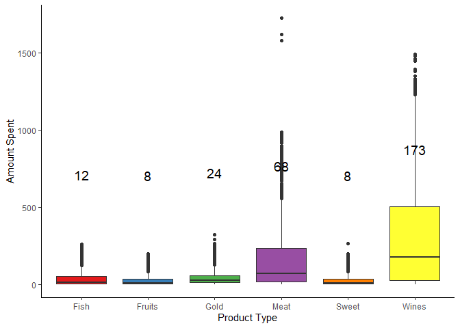
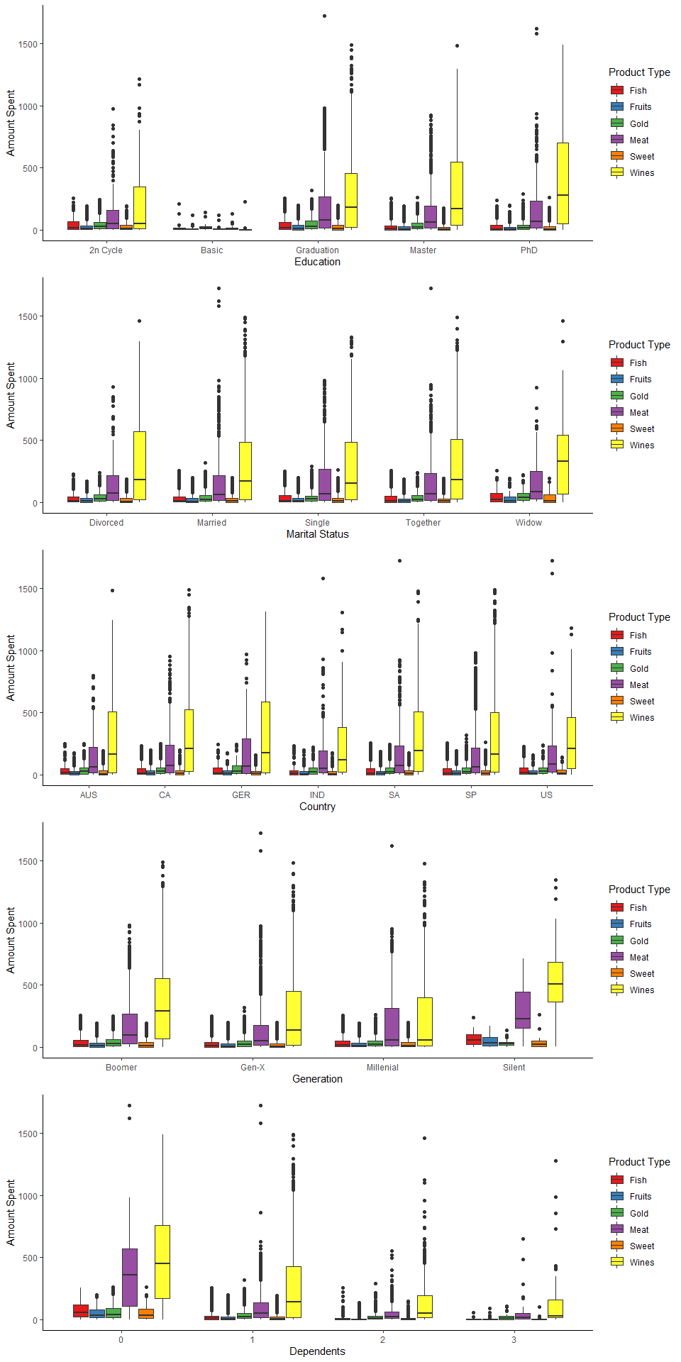
The best performing products overall is wine and then meat products. This is true even when you split the data by education, marital status, country, generation, and number of dependents.
Which marketing campaign is most successful?
# Overall
cmp <- mkt_data_ana %>%
  select(starts_with("Accepted")) %>% # Select the education and amount spent
  pivot_longer(starts_with("Accepted"), names_to = "variable", values_to = "response") %>%
  group_by(variable) %>%
  summarise(n = n(),
            sum = sum(response),
            success = sum/n,
            Percent = success*100) %>%
  mutate(variable = factor(variable),
         variable = fct_reorder(variable, desc(Percent)))# Wide to long format

ggplot(data = cmp, aes(x = variable, y = Percent, fill = variable)) +
  geom_bar(stat = "Identity") +
  labs(x = "Campaign", y = "Percent Accepted") +
  scale_fill_brewer(palette = "Set1") + # Change the colors +
  geom_text(aes(label = round(Percent, 1) %>% str_c("%")), vjust = -0.5) +
  coord_cartesian(clip = "off") +
  theme_classic() +
  theme(legend.position = "none")
Findings
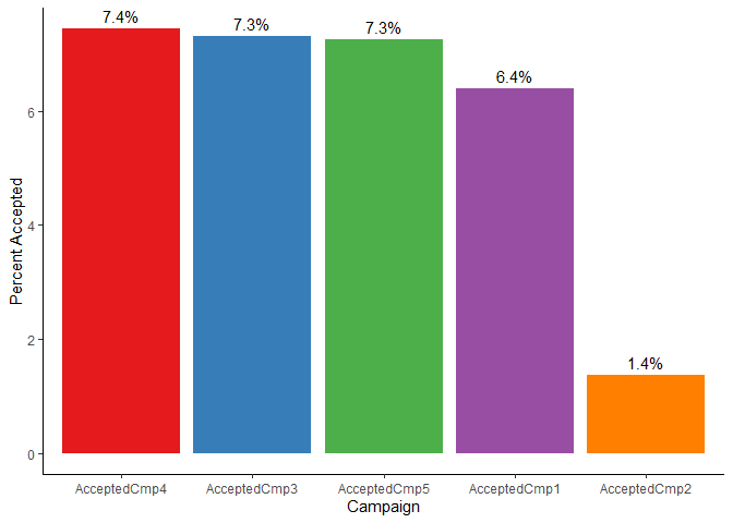
We can see that overall that the marketing campaigns are not doing well for increasing purchases of products. They have an average acceptance rate of 5.9555152.
Section 04: Statistical Analysis
Please run statistical tests in the form of regressions to answer these questions & propose data-driven action recommendations to your CMO. Make sure to interpret your results with non-statistical jargon so your CMO can understand your findings.
What factors are significantly related to the number of store purchases?
To run a regression, we need to first think about our data and see if we need to make changes to our data. This can be either removing data that is unnecessary or making some variables factors.
The following columns need to be removed because they are irrelevant or are related to other factors:
- ID
- Dt_Customer
- Year_Birth
- avg_pur
- tot_pur
- avg_mnt
- num_depends
- num_accepted
- Generation (age is better as continuous compared to a factor)
The following columns need to be removed because they have low data points: - Complain (Only 20/2203 responses)
The following columns need to be turned into a factor: - AcceptedCmp 1-5 (it is technically a categorical variable - 0 = No, 1 = Yes) - Response (0 = No, 1 = Yes)
Notes:
- Ideally we would know more information about what variables are key
- Be mindful of our dependent variable NumStorePurchases - it is a discrete, count variable
- Check to see if our regression is valid and does not violate assumptions of a linear model
- Remove any multicollinearity
# Remove the columns listed above
mkt_data_mod <- mkt_data_ana %>%
  select(-ID, -Dt_Customer, -Year_Birth, -avg_pur, -tot_pur, -avg_mnt, -tot_mnt, -Dependents, -num_accepted, -Generation, -Complain)

# Factor the Accepted Campaign variable
mkt_data_mod <- mkt_data_mod %>%
  mutate(AcceptedCmp1 = factor(AcceptedCmp1),
         AcceptedCmp2 = factor(AcceptedCmp2),
         AcceptedCmp3 = factor(AcceptedCmp3),
         AcceptedCmp4 = factor(AcceptedCmp4),
         AcceptedCmp5 = factor(AcceptedCmp5),
         Response     = factor(Response))

# Run the regression w/ all of the data
mod <- lm(NumStorePurchases ~ ., data = mkt_data_mod) # Run the model
step_mod <- step(mod, direction = "both", trace = 0) # Refine the model using stepwise selection using forward and backward selection
summary(step_mod) # See the estimates and the significance of each term
##
## Call:
## lm(formula = NumStorePurchases ~ Income + Kidhome + Recency +
##     MntWines + MntFruits + MntFishProducts + MntSweetProducts +
##     NumDealsPurchases + NumWebPurchases + NumCatalogPurchases +
##     NumWebVisitsMonth + AcceptedCmp3 + AcceptedCmp5 + AcceptedCmp1 +
##     AcceptedCmp2 + Response + Age + Yr_Customer, data = mkt_data_mod)
##
## Residuals:
##      Min       1Q   Median       3Q      Max
## -12.0254  -0.9466  -0.1353   0.8286   7.3590
##
## Coefficients:
##                       Estimate Std. Error t value Pr(>|t|)
## (Intercept)          4.013e+00  6.138e-01   6.537 7.77e-11 ***
## Income               6.551e-06  2.568e-06   2.551 0.010795 *
## Kidhome             -7.373e-01  1.112e-01  -6.633 4.13e-11 ***
## Recency             -3.411e-03  1.581e-03  -2.158 0.031072 *
## MntWines             3.799e-03  2.203e-04  17.246  < 2e-16 ***
## MntFruits            7.643e-03  1.530e-03   4.995 6.35e-07 ***
## MntFishProducts      4.108e-03  1.155e-03   3.557 0.000383 ***
## MntSweetProducts     5.422e-03  1.492e-03   3.634 0.000286 ***
## NumDealsPurchases    2.450e-01  2.748e-02   8.917  < 2e-16 ***
## NumWebPurchases      2.020e-01  2.212e-02   9.132  < 2e-16 ***
## NumCatalogPurchases -8.686e-02  2.440e-02  -3.560 0.000379 ***
## NumWebVisitsMonth   -3.277e-01  2.843e-02 -11.528  < 2e-16 ***
## AcceptedCmp31       -5.902e-01  1.799e-01  -3.280 0.001054 **
## AcceptedCmp51       -8.487e-01  2.177e-01  -3.899 9.96e-05 ***
## AcceptedCmp11       -3.412e-01  2.113e-01  -1.614 0.106597
## AcceptedCmp21        9.461e-01  4.043e-01   2.340 0.019378 *
## Response1           -8.267e-01  1.463e-01  -5.650 1.81e-08 ***
## Age                 -8.599e-03  4.028e-03  -2.135 0.032882 *
## Yr_Customer          1.947e-01  7.273e-02   2.676 0.007499 **
## ---
## Signif. codes:  0 '***' 0.001 '**' 0.01 '*' 0.05 '.' 0.1 ' ' 1
##
## Residual standard error: 2.087 on 2184 degrees of freedom
## Multiple R-squared:  0.5926, Adjusted R-squared:  0.5893
## F-statistic: 176.5 on 18 and 2184 DF,  p-value: < 2.2e-16
# See if there is any multicollinearity - if it is over 10, remove that and re-run the model
vif(step_mod)
##              Income             Kidhome             Recency            MntWines
##            2.120159            1.803195            1.058080            2.798209
##           MntFruits     MntFishProducts    MntSweetProducts   NumDealsPurchases
##            1.871458            2.006528            1.905682            1.414969
##     NumWebPurchases NumCatalogPurchases   NumWebVisitsMonth        AcceptedCmp3
##            1.855018            2.578222            2.400493            1.109714
##        AcceptedCmp5        AcceptedCmp1        AcceptedCmp2            Response
##            1.614667            1.353522            1.111027            1.372613
##                 Age         Yr_Customer
##            1.119597            1.253766
# Check to see if we violate any assumptions of the model
gvlma::gvlma(step_mod)
##
## Call:
## lm(formula = NumStorePurchases ~ Income + Kidhome + Recency +
##     MntWines + MntFruits + MntFishProducts + MntSweetProducts +
##     NumDealsPurchases + NumWebPurchases + NumCatalogPurchases +
##     NumWebVisitsMonth + AcceptedCmp3 + AcceptedCmp5 + AcceptedCmp1 +
##     AcceptedCmp2 + Response + Age + Yr_Customer, data = mkt_data_mod)
##
## Coefficients:
##         (Intercept)               Income              Kidhome
##           4.013e+00            6.551e-06           -7.373e-01
##             Recency             MntWines            MntFruits
##          -3.411e-03            3.799e-03            7.643e-03
##     MntFishProducts     MntSweetProducts    NumDealsPurchases
##           4.108e-03            5.422e-03            2.450e-01
##     NumWebPurchases  NumCatalogPurchases    NumWebVisitsMonth
##           2.020e-01           -8.686e-02           -3.277e-01
##       AcceptedCmp31        AcceptedCmp51        AcceptedCmp11
##          -5.902e-01           -8.487e-01           -3.412e-01
##       AcceptedCmp21            Response1                  Age
##           9.461e-01           -8.267e-01           -8.599e-03
##         Yr_Customer
##           1.947e-01
##
##
## ASSESSMENT OF THE LINEAR MODEL ASSUMPTIONS
## USING THE GLOBAL TEST ON 4 DEGREES-OF-FREEDOM:
## Level of Significance =  0.05
##
## Call:
##  gvlma::gvlma(x = step_mod)
##
##                       Value p-value                   Decision
## Global Stat        373.5557 0.00000 Assumptions NOT satisfied!
## Skewness             0.0619 0.80352    Assumptions acceptable.
## Kurtosis           278.2014 0.00000 Assumptions NOT satisfied!
## Link Function       91.3961 0.00000 Assumptions NOT satisfied!
## Heteroscedasticity   3.8963 0.04839 Assumptions NOT satisfied!
# Plot the data
plot(step_mod)
Findings
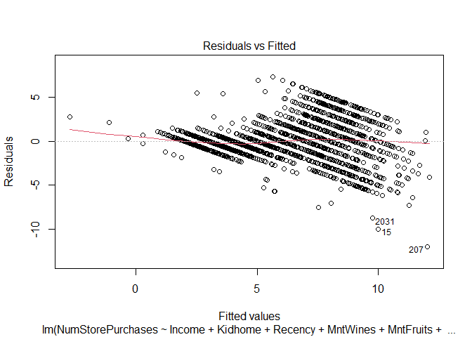
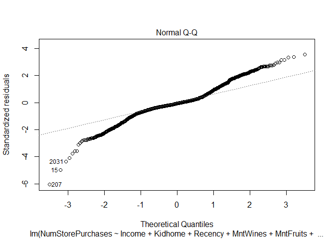
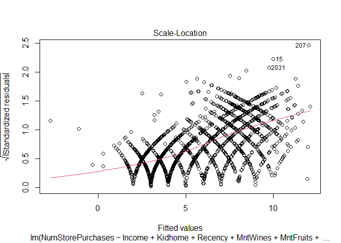
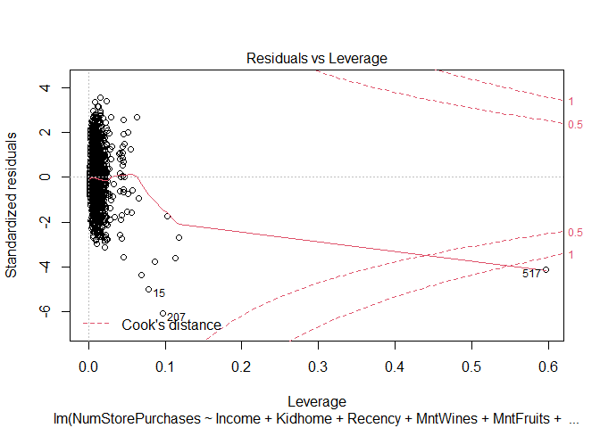
The model assumption check shows that we violate a number of important assumptions of the linear model - this makes it problematic when interpreting the results from this model.
- The residuals are not normally distributed - Kurtosis
- The dependent variable is not continuous, it is a count variable - Link Function
- Variance of the residuals is heteroscedastic - Heteroscedasticity
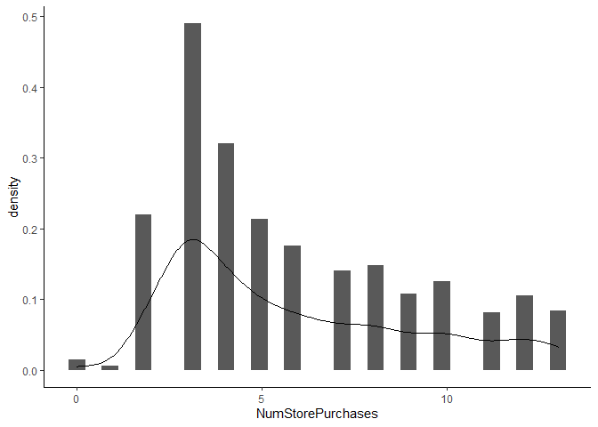
Therefore we need to use a different model approach to account for our dependent variable. Instead of a linear model, I will use a poisson model - an extension of the generalized linear family of models. The NumStorePurchases is a count variable and is discrete (cannot have half purchases) and it is bound by 0 (cannot have negative purchases).
Poisson model appraoch
# Plot the NumStorePurchases
ggplot(data = mkt_data_mod, aes(x = NumStorePurchases)) +
  geom_histogram(aes(y = ..density..)) +
  geom_density(alpha = 0.2) +
  theme_classic()
## `stat_bin()` using `bins = 30`. Pick better value with `binwidth`.
# Run the poisson model
poi_mod <- glm(NumStorePurchases ~ ., data = mkt_data_mod, family = "poisson") # Run the poisson regression
step_poi_mod <- step(poi_mod, direction = "both", trace = 0) # Refine the model by reducing AIC
summary(step_poi_mod) # Show the estimates of each term of out model
##
## Call:
## glm(formula = NumStorePurchases ~ Education + Income + Kidhome +
##     Recency + MntWines + MntFruits + MntFishProducts + MntSweetProducts +
##     NumDealsPurchases + NumWebPurchases + NumCatalogPurchases +
##     NumWebVisitsMonth + AcceptedCmp3 + AcceptedCmp5 + AcceptedCmp2 +
##     Response + Age + Yr_Customer, family = "poisson", data = mkt_data_mod)
##
## Deviance Residuals:
##     Min       1Q   Median       3Q      Max
## -5.8046  -0.4786  -0.0901   0.3572   2.8761
##
## Coefficients:
##                       Estimate Std. Error z value Pr(>|z|)
## (Intercept)          1.411e+00  1.258e-01  11.216  < 2e-16 ***
## EducationBasic      -2.402e-01  8.719e-02  -2.756 0.005860 **
## EducationGraduation -2.411e-02  3.286e-02  -0.734 0.463068
## EducationMaster     -2.346e-02  3.834e-02  -0.612 0.540580
## EducationPhD        -4.289e-02  3.752e-02  -1.143 0.252935
## Income               1.343e-06  4.357e-07   3.083 0.002047 **
## Kidhome             -1.924e-01  2.483e-02  -7.748 9.32e-15 ***
## Recency             -4.821e-04  3.137e-04  -1.537 0.124313
## MntWines             5.485e-04  3.886e-05  14.115  < 2e-16 ***
## MntFruits            1.061e-03  2.539e-04   4.179 2.92e-05 ***
## MntFishProducts      5.247e-04  1.945e-04   2.698 0.006980 **
## MntSweetProducts     4.803e-04  2.480e-04   1.937 0.052795 .
## NumDealsPurchases    5.382e-02  5.088e-03  10.578  < 2e-16 ***
## NumWebPurchases      3.968e-02  3.776e-03  10.509  < 2e-16 ***
## NumCatalogPurchases -1.402e-02  4.353e-03  -3.221 0.001277 **
## NumWebVisitsMonth   -6.964e-02  5.867e-03 -11.870  < 2e-16 ***
## AcceptedCmp31       -1.194e-01  3.803e-02  -3.140 0.001689 **
## AcceptedCmp51       -1.332e-01  3.671e-02  -3.629 0.000285 ***
## AcceptedCmp21        1.535e-01  6.857e-02   2.238 0.025210 *
## Response1           -1.399e-01  2.831e-02  -4.942 7.72e-07 ***
## Age                 -1.489e-03  7.900e-04  -1.884 0.059525 .
## Yr_Customer          4.102e-02  1.459e-02   2.811 0.004941 **
## ---
## Signif. codes:  0 '***' 0.001 '**' 0.01 '*' 0.05 '.' 0.1 ' ' 1
##
## (Dispersion parameter for poisson family taken to be 1)
##
##     Null deviance: 3920.3  on 2202  degrees of freedom
## Residual deviance: 1504.5  on 2181  degrees of freedom
## AIC: 9181.8
##
## Number of Fisher Scoring iterations: 5
# Run VIF on the poisson mod
vif(step_poi_mod)
##                         GVIF Df GVIF^(1/(2*Df))
## Education           1.288715  4        1.032214
## Income              1.705719  1        1.306032
## Kidhome             1.801772  1        1.342301
## Recency             1.051757  1        1.025552
## MntWines            2.541470  1        1.594199
## MntFruits           1.711784  1        1.308352
## MntFishProducts     1.839512  1        1.356286
## MntSweetProducts    1.755203  1        1.324841
## NumDealsPurchases   1.459051  1        1.207912
## NumWebPurchases     1.558442  1        1.248376
## NumCatalogPurchases 2.219829  1        1.489909
## NumWebVisitsMonth   2.498354  1        1.580618
## AcceptedCmp3        1.093605  1        1.045756
## AcceptedCmp5        1.603643  1        1.266350
## AcceptedCmp2        1.129813  1        1.062926
## Response            1.351491  1        1.162536
## Age                 1.110635  1        1.053867
## Yr_Customer         1.278895  1        1.130882
# Check for overdispersion
AER::dispersiontest(step_poi_mod) # we do not have overdispersion - model is OK!
##
##  Overdispersion test
##
## data:  step_poi_mod
## z = -13.175, p-value = 1
## alternative hypothesis: true dispersion is greater than 1
## sample estimates:
## dispersion
##  0.6635602
# Let's test our model using predictions

# First create the training protocol - K-fold Cross validation
set.seed(123)
train.control <- trainControl(method = "cv", number = 10, savePredictions = TRUE) # cv = crossvalidation

model <- train(NumStorePurchases ~ Education + Income + Kidhome +
    Recency + MntWines + MntFruits + MntFishProducts + MntSweetProducts +
    NumDealsPurchases + NumWebPurchases + NumCatalogPurchases +
    NumWebVisitsMonth + AcceptedCmp3 + AcceptedCmp5 + AcceptedCmp2 +
    Response + Age + Yr_Customer,
    data = mkt_data_mod,
    method = "glmnet",
    family = "poisson",
    trControl = train.control)

print(model)
## glmnet
##
## 2203 samples
##   18 predictor
##
## No pre-processing
## Resampling: Cross-Validated (10 fold)
## Summary of sample sizes: 1984, 1983, 1982, 1983, 1982, 1984, ...
## Resampling results across tuning parameters:
##
##   alpha  lambda       RMSE      Rsquared   MAE
##   0.10   0.004168224  5.073917  0.5742327  4.166468
##   0.10   0.041682241  5.073983  0.5744287  4.165806
##   0.10   0.416822412  2.328334  0.5003031  1.584382
##   0.55   0.004168224  5.073898  0.5742906  4.166591
##   0.55   0.041682241  5.074348  0.5750194  4.162689
##   0.55   0.416822412  2.444205  0.4707176  1.709032
##   1.00   0.004168224  5.073904  0.5743552  4.166469
##   1.00   0.041682241  5.075149  0.5740718  4.159876
##   1.00   0.416822412  2.745733  0.4339237  1.853523
##
## RMSE was used to select the optimal model using the smallest value.
## The final values used for the model were alpha = 0.1 and lambda = 0.4168224.
Findings
The results show that our model accounts for ~50% of the variance in the number of store purchases.
The average difference between the predicted and the actual number of purchases is 1.58 (MAE).
The main significant predictors are:
- Education Basic vs. 2nd Cycle (negative relationship)
- Income (positive relationship)
- Kidhome (negative relationship)
- Amount Wine/Fruits/Fish (positive relationship)
- Number of deals and web purchases (positive relationship)
- Number of catalog purchases (negative relationship)
- Number of web visits per month (negative relationship)
- Age (negative relationship)
- Accepted Campaign 2 vs. 1 (negative relationship)
- Accepted Campaign 3 vs. 1 (positive relationship)
- Accepted Campaign 5 vs. 1 (negative relationship)
- Year customer (positive relationship)
Positive relationship means that as the variable increases, the number of store purchases increases. Negative relationship means that as the variable increases, the number of store purchases decreases.
Main Takeaways
The average customer is…:
- Age: 52 years old
- Has been a customer for about 8 years
- Has an income of $5.1373^{4}
- Has at least 1 dependent
- Made a purchase from the company in the last 49
- They are most likely married
- They are most likely graduated
- They are most likely from Spain
The highest performing products are meat and wine. The CMO should decide on focusing on meat and wine or the underperforming products such as fish, fruits, gold, and sweets.
The underperforming channels are the catalog purchases and deals purchases. The CMO should decide whether or not to continue with the catalog purchases. The CMO should also reconsider the deals presented based on the type of products. If the company wants to increase sales of the underperforming products, they can create deals for fish, fruits, gold, and sweets.
The marketing campaigns are also missing their mark. The average acceptance rate for their marketing campaigns are 5.95%. The CMO should understand the needs and values of their customers (based on the profile above) to create marketing campaigns that either target their current audience or target a new audience.
